 |
Version 11.0.0
|
|
Version 11.0.0
|
Operation tracking tracks all API calls in WiredTiger as well as certain functions that are deemed important for performance, such as those in the eviction module. Tracking is performed by generating a log record when the execution enters and exits a tracked function. A log record contains a function name and its timestamp.
This tutorial will walk you through using operation tracking in WiredTiger on one of wtperf workloads: from preparing the workload for most effective data collection, to gathering, visualizing and interpreting the execution logs.
Analysis of WiredTiger JIRA tickets revealed that in diagnosing performance bugs engineers rely mostly on information that shows which functions were executed over time and across threads. They seek to find correlations between performance anomalies, such as long latencies or periods of low throughput, and events on these timelines. The purpose of operation tracking is to visualize the execution so that these correlations could be easily spotted.
Operation tracking allows you to put a pair of macros WT_TRACK_OP_INIT and WT_TRACK_OP_END into any function in WiredTiger whose invocation time you want to be measured and recorded. As your program runs, the WT_TRACK_OP_INIT macro will produce the function entry timestamp and WT_TRACK_OP_END macro will produce the function exit timestamp. These timestamps, along with the function name, will be recorded in a set of log files. It is typical to put the WT_TRACK_OP_INIT in the beginning of the function and the WT_TRACK_OP_END macro at every exit point from the function, but you can put them anywhere within the function body. The only condition required in order to correctly visualize the logs is that each WT_TRACK_OP_INIT has a matching WT_TRACK_OP_END. It is totally okay to insert tracking macros into nested functions.
The answer depends on your workload, and how many functions you track. For wtperf suite the largest overhead of 30% was observed on the CPU-bound workload small-btree. For I/O-bound workloads, such as evict-btree-stress-multi, the overhead is negligible, unless you decided to track short frequently executed functions.
Modify your benchmark so that it produces the desired behavior with as little running time as possible. The longer the benchmark runs the more data it will produce, and the more difficult it will be for you to go over all this data.
In our running example with the evict-btree-stress-multi.wtperf workload, we separate the database creation phase from the work phase. We first create the database with operation tracking disabled. Then we enable operation tracking and run the work phase. So operation tracking logs are generated during the work phase only. We also reduce the work phase to 30 seconds, to make sure that the volume of information is manageable.
To generate data visualizations, you will need the python modules bokeh, matplotlib and pandas installed. You can install them via the following commands (if you don't use pip modify for your python module manager):
pip install bokeh matplotlib pandas
To enable operation tracking, you need to add the following option to your connection configuration string.
operation_tracking=(enabled=true,path=.)
For example, if you are running wtperf, you would add it to the conn_config string:
./wtperf -C conn_config="operation_tracking=(enabled=true,path=.)"
The "path" argument determines where the log files, produced by operation tracking, will be stored. Now you can run your workload.
After the run is complete, the path directory will have a bunch of files of the following format:
optrack.00000<pid>.000000000<sid>
and the file
optrack-map.00000<pid>
where pid is the process ID and sid is the session ID.
The first kind of files are the actual log files. The second is the map file. Log files are generated in the binary format, because this is a lot more efficient than writing strings, and the map file is needed to decode them.
Now the binary log files need to be converted into the text format. To do that use the script wt_optrack_decode.py in the WiredTiger tree. We will refer to the path to your WiredTiger tree as WiredTiger. Suppose that the process ID that generated the operation tracking files is 25660. Then you'd run the decode script like so:
% python WT/tools/optrack/wt_optrack_decode.py -m optrack-map.0000025660 optrack.0000025660.00000000*
As the script runs you will see lots of output on the screen reporting the progress through the parsing process. One kind of output you might see is something like this:
TSC_NSEC ratio parsed: 2.8000
This refers to the clock cycles to nanoseconds ratio encoded into the log files. In the example above, we had 2.8 ticks per nanosecond, suggesting that the workload was run on a 2.8 GHz processor. This ratio is used later to convert the timestamps, which are recorded in clock cycles for efficiency, to nanoseconds.
In the end, you should see lots of output files whose names look like the optrack log files, but with the suffixes -internal.txt and -external.txt. The "internal" files are the log files for WiredTiger internal sessions (such as eviction threads). The "external" files are for the sessions created by the client application.
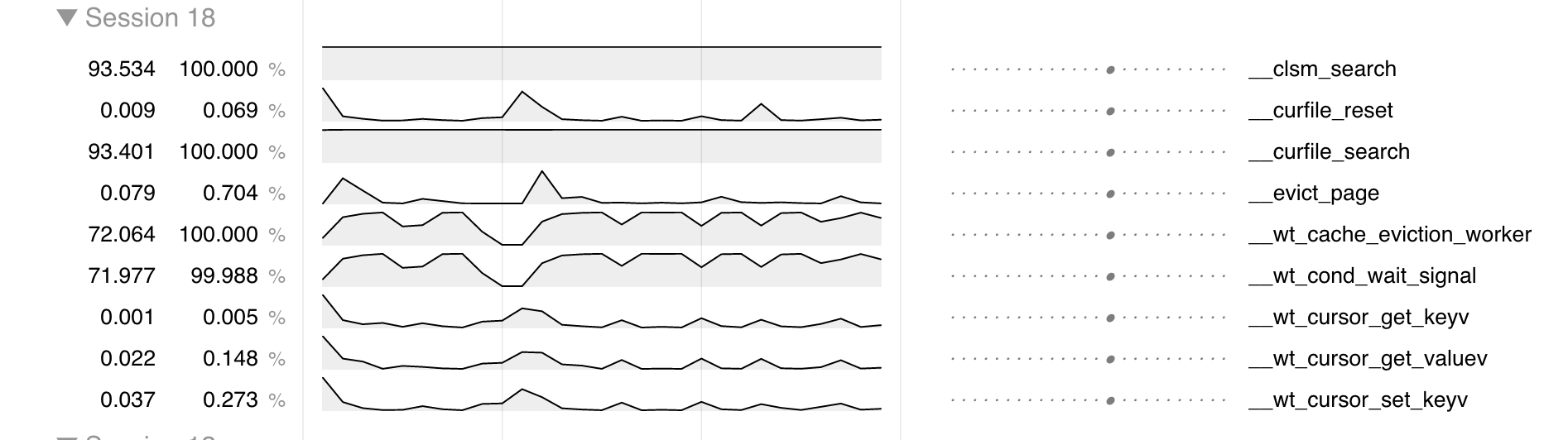
There are two ways to view operation tracking data, besides manually plowing through the log files. The quickest way is to generate CSV files viewable with t2 – MongoDB's internal tool. With t2, you can view the frequency of tracked operations across time and across threads, like this:
To produce a CSV file that can be loaded directly into t2, run the following command:
% WT/tools/optrack/optrack_to_t2.py optrack.0000025660.00000000*.txt
The second option is to use a script that will help you locate latency spikes – invocations of operations that took an unusually long time – and visually examine per-thread operation logs around those spikes. To obtain such a visualization, use the script find-latency-spikes.py located in the tools/optrack directory of the WiredTiger tree. To process the text files in our example, you run this script as follows:
% WT/tools/optrack/find-latency-spikes.py optrack.0000025660.00000000*.txt
As the script runs, you will probably see messages similar to this one:
Processing file optrack.0000025660.0000000026-external.txt
Your data may have errors. Check the file .optrack.0000025660.0000000026-external.txt.log for details.
This means that as the script was processing the log file, it found some inconsistencies, for example there was a function entry timestamp, but no corresponding function exit, or vice versa. Sometimes these errors are benign. For example, the log file will never have an exit timestamp from a session-closing function, because operation tracking is torn down as the session closes. In other cases, an error may indicate that there is a mistake in how the operation-tracking macros were inserted. For example, the programmer may have forgotten to insert a macro where there is an early return from a function. Examining the log file mentioned in the error message will give you more details on the error.
The data processing script will not fail or exit if it encounters these error messages, it will proceed despite them, attempting to visualize the portion of the log that did not contain the errors. The function timestamps implicated in the errors will simply be dropped.
At the very end of the processing, you will see messages like this:
Normalizing data...
Generating timeline charts... 99% complete
Generating outlier histograms... 100% complete
This is how you know the processing has completed. The script takes a while to run, but it is parallelizable, so that is something that can be done in the future to speed it up.
In the directory where you ran the data processing script, you will have the file WT-outliers.html and the directory BUCKET-FILES to which that HTML file refers. If you would like to look at the visualization on another machine, transfer both the HTML file and the directory to that machine. Otherwise, just open WT-outliers.html locally in your browser.
To get an idea of what kind of output you will see, take a look at this example data generated by the workload described earlier in this tutorial. Please open the URL, because we will now walk over what it shows.
The main page shows a number of outlier histograms. Each histogram corresponds to a function that was tracked by the operation tracking system in WiredTiger. The x-axis shows the execution timeline (in nanoseconds). The y-axis shows how many abnormally long executions of the function occurred during very period of the execution.
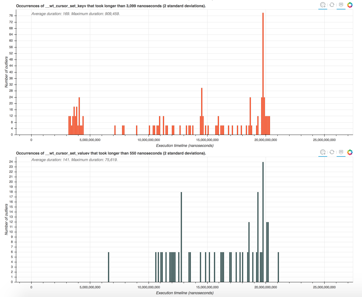
You can click on outlier bars and look at the detailed visualization of the period during which the abnormally long function invocations occurred. But before we do that, let's talk about what is considered an "outlier" or an "abnormally long execution" and how to control these thresholds. As annotations on the histograms show, by default a function invocation is considered an outlier if its duration is longer than two standard deviations above average. (The average is computed for this function over the entire execution). If you would like a more precise control of outlier thresholds, you can do that in a configuration file that is read by the execution script.
Before we talk about other visualization screens, let's actually generate a visualization with some more meaningful outlier thresholds than two standard deviations. This way, it will be easier to navigate the data, and we will be able to observe some very interesting behavior that gives us a clue as to why eviction is sometimes slow. (If you can't wait to find out, skip over the next step.)
Let's learn how to configure custom outlier thresholds. The easiest way to begin is to grab a sample configuration file and edit it to your needs:
% cp WT/tools/optrack/sample.config .
Here is how that file looks:
# Units in which timestamps are recorded
1000000000
# Outlier threshold for individual functions
__curfile_reset 100 ms
__curfile_search 50 ms
__curfile_update 3 ms
__evict_lru_pages 75 ms
__evict_lru_walk 20 ms
__evict_page 75 ms
__evict_walk 20 ms
__wt_cache_eviction_worker 10 ms
__wt_cond_wait_signal 5 s
__wt_cursor_set_valuev 10 ms
In that file all lines prefixed with a # are comments.
The first non-comment line specifies the units in which your timestamps are recorded. The units are specified by providing a value indicating how many time units there are in a second. By default operation scripts generate timestamps in nanoseconds, hence you see a value of 1000000000 on the first line in our sample file. If your time units were, say, milliseconds, you'd change that value to 1000, and so on.
The remaining non-comment lines in the file provide the outlier thresholds for any functions you care to have a custom threshold. The format is:
<function name> <value> <unit>
For example, to specify a threshold of 15 milliseconds for the __wt_cache_eviction_worker function, you'd insert the following line:
__wt_cache_eviction_worker 15 ms
Valid units are nanoseconds (ns), microseconds (us), milliseconds (ms) and seconds (s).
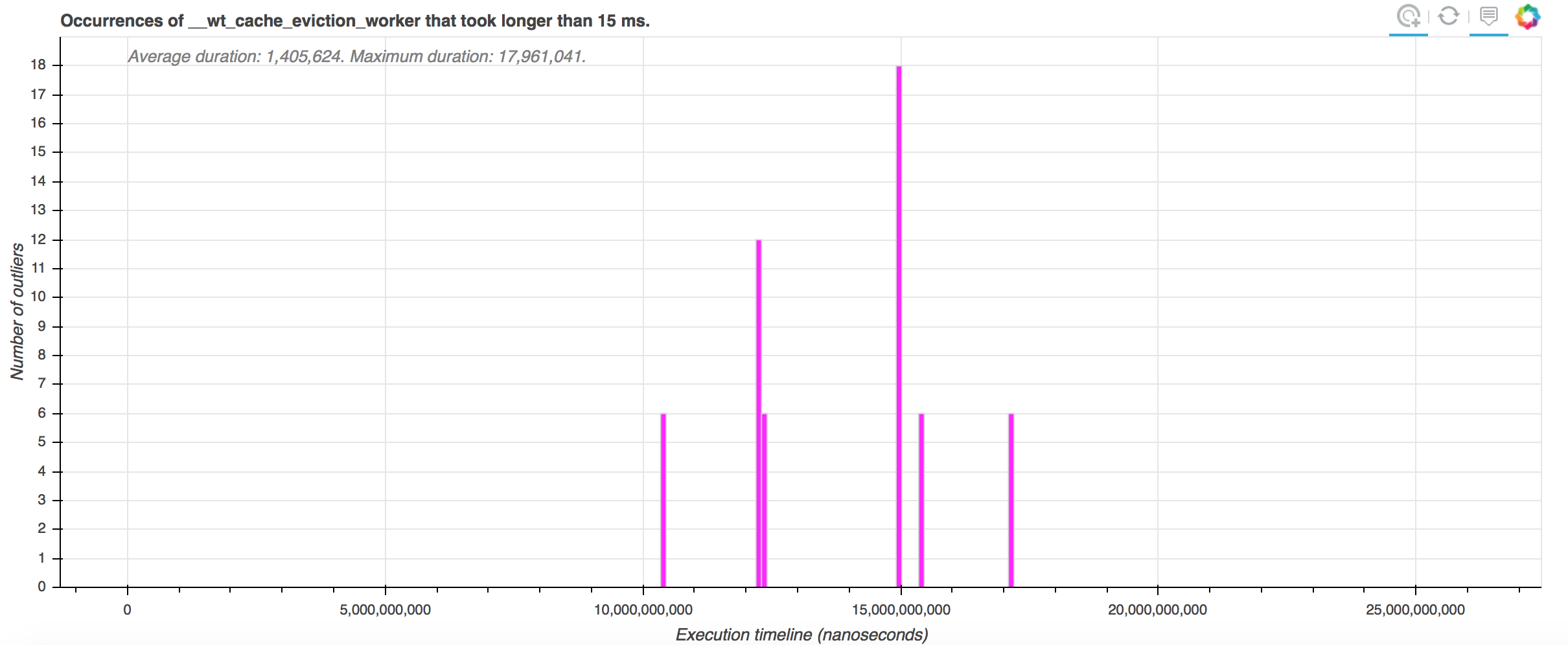
If you don't specify a threshold for a function the default of two standard deviations will be used. Let's actually configure some more meaningful outlier thresholds in our sample.config file and re-run the visualization script. Here is the modified sample.config:
# Units in which timestamps are recorded
1000000000
# Outlier threshold for individual functions
__curfile_search 30 ms
__evict_lru_pages 250 ms
__evict_lru_walk 1 ms
__evict_page 15 ms
__evict_walk 1 ms
__wt_cache_eviction_worker 15 ms
__wt_cond_wait_signal 10 s
We rerun the data processing script with the configuration file argument, like so:
% WT/tools/optrack/find-latency-spikes.py -c sample.config optrack.0000025660.00000000*.txt
The new charts can be accessed here.
Let's examine the visualized data in more detail. Please click on this URL:
Although I insert the screenshots here, you will have more fun if you access it directly.
Now you can see the outlier charts complying with the configuration parameters we supplied. For example, on the chart for the __wt_cache_eviction_worker, we see only the intervals where that function took longer than 15 ms to complete.
Let's click on one of those intervals to examine what happened there. I am going to click on the tallest bar in the chart, which will take me to a detailed output of function call activity by thread for interval 137 at this URL.
There is a lot of graphics there, so the URL might take a few seconds to load.
At the very top of the page you see a small navigation bar. The bar tells you where you are in the execution (the red marker). By clicking on other intervals within the bar you can navigate to other intervals. For example, if you wanted to look at the execution interval located after the current one, you will just click on the white bar following the current, red-highlighted, bar.

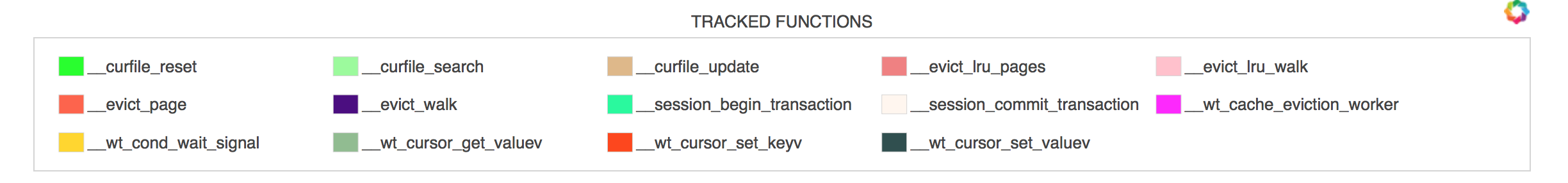
Next you see a legend that shows all functions that were called during this execution interval and their corresponding colors.
Then you will see the most interesting information: function calls across threads that occurred during this period. Durations and hierarchy of function calls is preserved, meaning that longer functions will be shown with longer bars and if function A called function B, B will be shown on top of A.
By hovering over the colored bars corresponding to functions, you will see a box appear telling you the name of the function, how long it took and its original timestamp in your operation tracking log file. This way, if you are suspicious about the correctness of your log or want to go back to it for some reason, you know what to look for.
In our example visualization, if we scroll down to the function sequences for external threads, we will quickly see a few instances where __wt_cache_eviction_worker took longer than 15 ms, for example here:
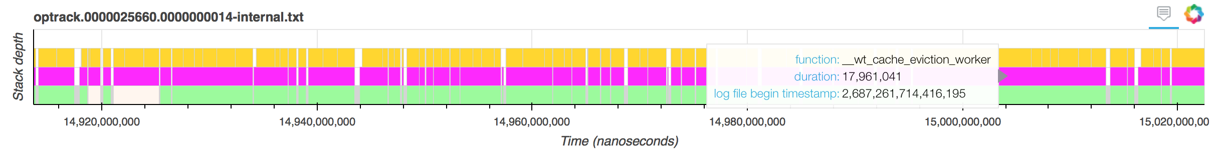
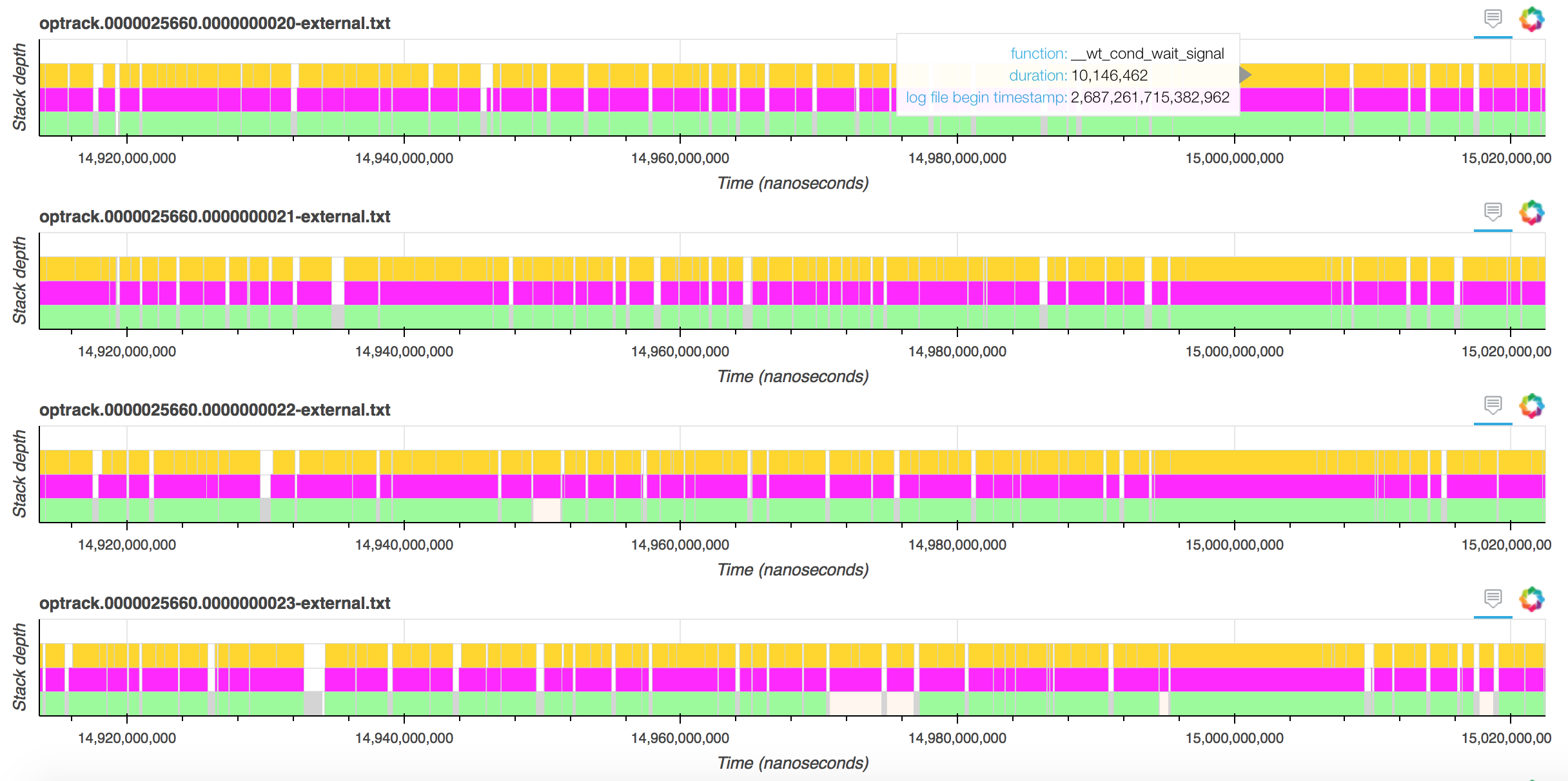
As we can see, the threads are simply waiting on the condition variable inside the eviction worker. To try and understand why, we might want to scroll up and look at the activity of internal threads during this period. Interestingly enough, most of the internal threads are also waiting on the condition variable during this period.
Looking at the internal thread with session id 1 shows something suspicious.
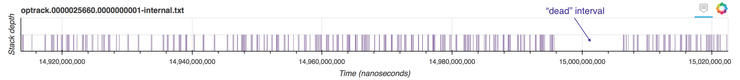
During this period where all threads are waiting, this thread shows no activity at all, whereas prior and after that "dead" period it was making regular calls to __evict_walk. Perhaps that thread was unscheduled or stopped calling __evict_walk for other reasons. Perhaps other threads were dependent on work performed within __evict_walk to make forward progress.
To better understand why __evict_walk was interrupted for almost 10ms we might want to go back and insert operation tracking macros inside the functions called by __evict_walk, to see if the thread was doing some other work during this time or was simply unscheduled.
Operation tracking is great for debugging performance problems where you are interested in understanding the activity of the workload over time and across threads. To effectively navigate large quantities of data it is best to reproduce your performance problem in a short run.